MIDAS regrids to a fresh uniform mesh after every interface movement (see Equations), so there’s no persistent mesh-quality issue to manage the way there is in a fixed-grid code - the two knobs that matter are grid resolution (nx_A/nx_B) and the time step(governed by CFL, indirectly).

Grid resolution: nx_A, nx_B

The six shipped examples all use nx_A = nx_B = 200, which is generally enough to resolve the diffusion profile’s curvature near the interface (where gradients are steepest) without the grid dominating runtime. If you’re not sure a given configuration is resolved:

1. Run once at the shipped resolution, note R.S_final and R.tALuHf1_final (or whichever output you care about).
2. Double nx_A/nx_B, rerun, compare. If the answer barely moves, you were already resolved; if it moves a lot, keep doubling until it stops moving.

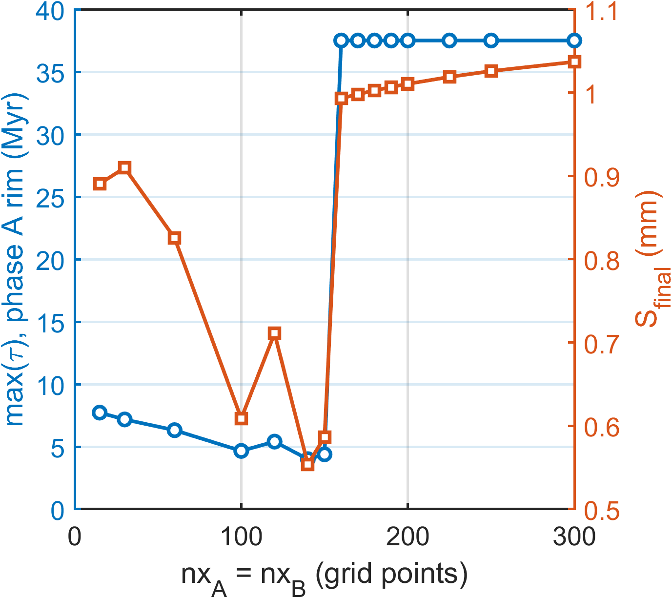
A real convergence check for Example1_Baseline: nx_A = nx_B at 15 points from 15 up to 300, densely sampled around the transition. This isn’t smooth convergence - it’s a sharp threshold between nx=150 and nx=160: below it, both diagnostics are not just off but genuinely erratic (S_final swings 0.61 -> 0.71 -> 0.55 -> 0.59 mm between nx=100 and nx=150, no visible trend); at nx=160 and above, both jump to and stay on a flat, stable plateau all the way to nx=300. The shipped examples’ default of nx_A = nx_B = 200 sits safely inside that stable plateau, with headroom to spare - and this is exactly the kind of jump the doubling recipe above is meant to catch, since the erratic region below threshold could easily look like “probably fine” from a single under-sampled check.

The CI smoke test deliberately runs at nx_A = nx_B = 15 - fast enough for every push, but not resolved enough to trust scientifically; it exists only to catch the pipeline breaking outright (see Benchmarks for what happens to the mass-balance/misfit diagnostics at full resolution, which the smoke test doesn’t check).

lxB_factor (matrix length relative to crystal length) interacts with this: a larger matrix reservoir at the same nx_B means coarser absolute spatial resolution in phase B specifically, since dx_B = lxB/(nx_B-1).

Time step

There’s no separate time-step parameter to tune directly - dt is fully adaptive, taken as the smallest of several stability/accuracy timescales (diffusion, interface-kinetic relaxation, and interface advection, each evaluated per tracked species) every step, scaled by CFL (see Equations). Two consequences worth knowing:

• CFL is not the classical explicit-scheme CFL number. Diffusion here is unconditionally stable (implicit), so CFL values up to 500 (the shipped default) are normal and fine - it mainly governs how far the interface is allowed to move in one step, not numerical stability. Lowering it gives a smoother, more finely time-resolved run at the cost of more steps; it’s not needed for correctness.
• CFL must be strictly greater than 0. Every stability/accuracy timescale that dt is built from is scaled directly by CFL (not divided by it), so CFL = 0 makes dt = 0 - the model time never advances, and the run hangs indefinitely rather than erroring or producing a wrong answer. A negative CFL is equally invalid. There’s no built-in check for this (as of this writing) - if a run seems to hang forever with no output and no error, check this first.

• nStepsMin guards against the opposite failure mode: a near-stagnant run (growth velocity $\approx 0$) where the advection timescale $\Delta x/

  v

  $ is effectively infinite, which would otherwise let a single step jump straight to t_tot with no recorded history in between. Raise it if a run’s store_history output looks too coarse during a slow-growth phase specifically.

If a run throws 'Reduce CFL, growth >> dxB' (or the resorption equivalent), the interface moved more than one full grid cell in a single step - lower CFL rather than raising nx_A/nx_B (the latter makes the problem worse, since a finer grid means a smaller dx to overshoot).