
MIDAS solves growth/resorption of a mineral couple (phase A, the crystal; phase B, the surrounding matrix) subject to diffusion and interface kinetics, and calculates apparent $^{176}$Lu-$^{176}$Hf ages from the result. This page summarizes the physical/chemical background and the numerical implementation, following the structure of the project’s own technical documentation (Stroh & Moulas, in prep.) and the code (MIDAS_Main.m) directly - every equation below has a corresponding line or block there.
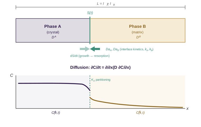
The symbols this page uses, laid out spatially: phase A and B share one domain of total length $L=l_A+l_B$, each with its own diffusivity; the interface $S(t)$ moves according to the growth/resorption velocity $dS/dt$ and is governed by the Damköhler numbers $\mathrm{Da}_A$, $\mathrm{Da}_B$ (interface rate constants $k^A$, $k^B$); concentrations on either side are tied together by the partition coefficient $K_D$.
Isotopic decay and apparent ages
Unstable isotopes decay from a parent $N_P$ into a daughter $N_D$:
\[N_P(t) = N_P(0)\, e^{-\lambda t}, \qquad N_D(t) = N_D(0) + N_P(0)\big(1-e^{-\lambda t}\big)\]with decay constant $\lambda$. MIDAS implements the $^{176}$Lu-$^{176}$Hf system: $^{176}$Lu decays into $^{176}$Hf with $\lambda = 1.867\times 10^{-11}\ \mathrm{yr^{-1}}$ (Söderlund et al., 2004), and the initial $^{176}$Hf content of phase A is assumed zero - all $^{176}$Hf in the crystal is produced in situ. The ratio of daughter to parent then gives the apparent age at any point:
\[\tau = \frac{1}{\lambda}\ln\!\left(\frac{N_D(t) - N_D(0)}{N_P(t)} + 1\right)\]evaluated pointwise across the whole profile every recorded step (tALuHf1/tBLuHf1 in the code). Away from the diffusively-reset rim, $\tau \approx t$; near the rim (or after resorption/regrowth), $\tau$ diverges from the true model time - that divergence (R.misfitApparent_final) is a direct diagnostic of how much a naive single-point age would be biased by diffusion.
Diffusion modelling
Solid-state diffusion follows Fick’s second law,
\[\frac{\partial C}{\partial t} = \frac{\partial}{\partial x}\!\left(D\,\frac{\partial C}{\partial x}\right)\]where $D = D(T,P,C)$. For multicomponent diffusion (e.g. in garnet), this generalizes to a diffusivity matrix (Onsager formulation) that couples all tracked components together - relevant when complex zoning results from the interplay between several elements. MIDAS currently simplifies this to binary Fe-Mg interdiffusion for the major-element system (the multicomponent form is noted here for context/future extension, not implemented). The effective binary Mg-Fe interdiffusion coefficient follows Chakraborty & Ganguly (1991), combined via the Manning (1968) formulation as given in Ganguly et al. (2001):
\[D_i = D_{0,i}\, e^{-Q_i/RT}, \qquad D_{\mathrm{Mg\text{-}Fe}} = \frac{D_{Mg}\,D_{Fe}}{X_{Mg}D_{Mg} + (1-X_{Mg})D_{Fe}}\]Mn, Lu, and Hf are each treated as independent tracer diffusivities (same Arrhenius form, first term of the equation above):
| Cation | $D_0$ (cm$^2$/s) | $Q$ (cal/mol, +$P$-dependence) | Reference |
|---|---|---|---|
| Mg$^{2+}$ | $1.11\times10^{-3}$ | $67997 + 0.1276\,P_{bar}$ | Chakraborty & Ganguly (1991) |
| Fe$^{2+}$ | $6.36\times10^{-4}$ | $65824 + 0.1363\,P_{bar}$ | Chakraborty & Ganguly (1991) |
| Mn$^{2+}$ | $5.15\times10^{-4}$ | $60569 + 0.1463\,P_{bar}$ | Chakraborty & Ganguly (1991) |
| Lu$^{3+}$ | $1.15\times10^{-5}$ | 272.8 kJ/mol + 10.8 cm$^3$/mol $\times P$ | Bloch et al. (2015) |
| Hf$^{4+}$ | $2.37\times10^{-5}$ | 291.6 kJ/mol + 12.5 cm$^3$/mol $\times P$ | Bloch et al. (2015) |
The user sets phase-A diffusivities as input; phase-B diffusivities are set relative to phase A via a fixed ratio (DRG, DRG_LuHf, DRG_Mn) rather than their own independent T-dependence - matrix diffusion is numerically homogenized ($D_B = \overline{D_A}\cdot\mathrm{DRG}$), so this ratio is an effective contrast rather than a literal mineral-specific diffusivity. All diffusivities are converted to mm$^2$/Myr internally.
At the interface, $C_A^{int}$ and $C_B^{int}$ are not independently known - two more relations close the system: the partition coefficient and a local flux balance (see Growth modelling below):
\[K_D = \frac{C_A^{int}}{C_B^{int}}, \qquad (C_B^{int}-C_A^{int})\,v = J_B - J_A, \qquad J = -D\,\frac{\partial C}{\partial x}\]Reaction modelling and interface kinetics
Interface reactions are treated with first-order kinetics (Lasaga, 1986): the interface composition relaxes toward its local equilibrium value at a rate set by a kinetic constant $\kappa$,
\[\frac{dC}{dt} = -\kappa\,(C - C_{eq}) \quad\Longrightarrow\quad C(t+\Delta t) = C_{eq} + \big(C(t)-C_{eq}\big)\,e^{-\kappa\,\Delta t}\]solved in closed form every step (unconditionally stable regardless of $\Delta t$), independently for each side ($\kappa_A$ from DamA, $\kappa_B$ from DamB) and for every tracked species. $\kappa$ is expressed through the (dimensionless) Damköhler number (Damköhler, 1936),
comparing the diffusion timescale ($L^2/D$) to the reaction timescale ($1/\kappa$). $\mathrm{Da} \gg 1$: interface reaction is fast relative to diffusion, so the system approaches local equilibrium at the interface and diffusion controls the overall rate (diffusion-limited regime). $\mathrm{Da} \ll 1$: the interface reaction itself is the bottleneck (interface-limited regime, the model’s namesake case) and the interface composition can lag well behind local equilibrium. $\mathrm{Da}\sim 1$: a mixed regime where both matter. DamA/DamB set this directly; MIDAS’s own defaults (DamA = DamB = 1e3) sit deep in the diffusion-limited limit for the major elements, i.e. close to local equilibrium at the interface.
Growth modelling (the chemical Stefan condition)
The crystal can only grow or resorb with a single velocity $v$, shared by every tracked species. $v$ is solved directly from the major-element flux balance at the interface (the chemical Stefan condition, following the approach of Stroh et al., 2025):
\[v = \frac{J_B - J_A}{C_B^{int} - C_A^{int}}\]with $v>0$ growth (phase A expands, phase B is consumed) and $v<0$ resorption (the reverse). Once $v$ is known from the major-element solve, it is reused - not re-derived - to solve each trace element’s own interface boundary values from its own $K_D$ and flux balance (see Diffusion modelling above; solveBC in the code). If a trace-element boundary value would go negative (possible at extreme DamA/DRG corners of parameter space), the run stops early and returns the last self-consistent step (R.stoppedEarly, R.stopReason) instead of continuing with an unphysical state.
Apparent age determination
MIDAS offers three ways to assign an age:
- Model time itself - trivial, but only meaningful for interpreting the model’s own internal consistency (see Benchmarks).
- Single-point apparent age, Eq. (above) - evaluated at every node, every recorded step.
-
Isochron age (two-point regression, e.g. Faure & Mensing, 2005): assuming a cogenetic mineral pair sharing one true age $t$ and one initial daughter content, a non-radiogenic reference field $\mathrm{Hf_r}$ (never touched by decay, carried alongside Hf purely to normalize the isochron axes) gives
\[X = \frac{\mathrm{Lu}}{\mathrm{Hf_r}}, \qquad Y = \frac{\mathrm{Hf}}{\mathrm{Hf_r}}, \qquad Y = Y_{ref} + \big(e^{\lambda t}-1\big)\,(X - X_{ref})\]A line is fit (MATLAB’s
polyfit/polyval) through one point from phase A (rim, core, bulk, or everyisoNskip-th node) and one external reference point set byisoRefMode:'bulk'(phase B’s volume-weighted average),'core'(phase B’s node farthest from the interface, i.e. least disturbed by diffusion), or'wholerock'(volume-weighted average of A+B together). The age follows from the fitted slope, $t = \ln(\mathrm{slope}+1)/\lambda$. Isochrons are always computed for phase A’s core, rim, and bulk (plus whichever of those is oldest, “max”); additional profile points are optional (isoNskip, plotted ifisoShowProfile = 1).HfiBrefis phase B’s initial $^{177}$Hf content (ppm), used only to fix the normalizing ratio (chondritic $^{176}$Lu/$^{177}$Hf $\approx 0.279$; Faure & Mensing, 2005) - it does not otherwise affect the diffusion/growth solution.
Numerical implementation
An implicit (backward Euler) finite-difference/finite-volume scheme is used throughout, for unconditional stability with respect to $D$. Both phases share a geometry-dependent 1-D diffusion equation, parameterized by ndim ($n$: 1 planar, 2 cylindrical, 3 spherical):
discretized on a finite-volume grid (nx_A/nx_B nodes per phase) and solved directly with the Thomas algorithm (small, order-100-unknown tridiagonal systems, rebuilt every step). The outer boundary condition (NBC) is Neumann (no-flux, a closed system) or Dirichlet (fixed at the initial value, simulating an infinite open-system reservoir); Dirichlet is required whenever ndim = 2 or 3 (cylindrical/spherical). The interface-facing boundary of each phase is always Dirichlet, set by the kinetic relaxation described above.
| Adaptive time stepping: at every step, MIDAS compares the timescales for interface relaxation (reaction, $1/\kappa$), diffusion ($\Delta x^2/D$), and interface advection ($\Delta x/ | v | $) - separately for every tracked major and trace element/isotope - and takes the smallest, scaled by the CFL number: |
CFL is conventionally $<1$ for explicit schemes, but since diffusion here is unconditionally stable, MIDAS uses values up to 500 for speed - the $\Delta x/ |
v | $ term (scaled by an internal factor of 0.4) is what actually keeps growth/resorption from overshooting a full node per step. nStepsMin bounds $\Delta t$ from above so a near-stagnant run ($v\to0$) still resolves a time history instead of jumping to $t_{tot}$ in one step. |
Regridding: after the interface moves, both grids are resampled with a shape-preserving cubic interpolant (pchip) onto fresh uniform grids (following Stroh et al., 2025’s approach) - except when the movement is below microStepTol (default $10^{-12}$ mm), in which case only the boundary node is updated in place, skipping the resample entirely. This resampling is the main source of the small mass-balance drift discussed in Benchmarks.
Output: MIDAS_Main returns everything in one struct R. Key fields: R.xA_final/R.xB_final (final spatial grids, mm), R.CA_final/R CB_final (final major-element profiles), R.CALu_final/R.CAHf_final (final Lu/Hf profiles, phase A), R.tALuHf1_final (final apparent-age profile, phase A), R.S_final (final interface position, mm), R.t_final (elapsed model time, Myr), and R.params (a copy of the input struct used for the run). If store_history = 1, the full time series is also stored, generally as <field>rec (e.g. R.CArec, R.Srec, R.trec) - the apparent-age history is the one exception, stored as R.tA1/R.tB1. SeeAPI Reference for the complete field list.
References
- Bloch, E., Ganguly, J., Hervig, R., and Cheng, W.: $^{176}$Lu-$^{176}$Hf geochronology of garnet I: experimental determination of the diffusion kinetics of Lu$^{3+}$ and Hf$^{4+}$ in garnet, closure temperatures and geochronological implications, Contrib. Mineral. Petrol., 169, 12, doi:10.1007/s00410-015-1109-8, 2015.
- Chakraborty, S. and Ganguly, J.: Compositional Zoning and Cation Diffusion in Garnets, in: Diffusion, Atomic Ordering, and Mass Transport, Springer US, 120-175, doi:10.1007/978-1-4613-9019-0_4, 1991.
- Damköhler, G.: Einflüsse der Strömung, Diffusion und des Wärmeüberganges auf die Leistung von Reaktionsöfen, Z. Für Elektrochem. Angew. Phys. Chem., 42, 846-862, doi:10.1002/bbpc.19360421203, 1936.
- Faure, G. and Mensing, T. M.: Isotopes: Principles And Applications, 3rd ed., WILEY, 2005.
- Ganguly, J., Hensen, B. J., and Cheng, W.: Reaction texture and Fe-Mg zoning in granulite garnet from Søstrene Island, Antarctica, J. Earth Syst. Sci., 110, 305-312, doi:10.1007/BF02702897, 2001.
- Kohn, M. J.: Models of garnet differential geochronology, Geochim. Cosmochim. Acta, 73, 170-182, doi:10.1016/j.gca.2008.10.004, 2009.
- Lasaga, A. C.: Metamorphic reaction rate laws and development of isograds, Mineral. Mag., 50, 359-373, doi:10.1180/minmag.1986.050.357.02, 1986.
- Söderlund, U., Patchett, P. J., Vervoort, J. D., and Isachsen, C. E.: The $^{176}$Lu decay constant determined by Lu-Hf and U-Pb isotope systematics of Precambrian mafic intrusions, Earth Planet. Sci. Lett., 219, 311-324, doi:10.1016/S0012-821X(04)00012-3, 2004.
- Stroh, A., Aellig, P. S., and Moulas, E.: Numerical modelling of diffusion-limited mineral growth for geospeedometry applications, Geosci. Model Dev., 18, 10203-10220, doi:10.5194/gmd-18-10203-2025, 2025.